Routing Algorithms

Distance vector Routing

A distance-vector routing (DVR) protocol requires that a router inform its neighbors of topology changes periodically. Historically known as the old ARPANET routing algorithm (or known as Bellman-Ford algorithm).

Bellman Ford Basics – Each router maintains a Distance Vector table containing the distance between itself and ALL possible destination nodes. Distances,based on a chosen metric, are computed using information from the neighbors’ distance vectors.

Information kept by DV router –

• Each router has an ID
• Associated with each link connected to a router,
• there is a link cost (static or dynamic).
• Intermediate hops

Distance Vector Table Initialization –

• Distance to itself = 0
• Distance to ALL other routers = infinity number.

Distance Vector Algorithm –

1. A router transmits its distance vector to each of its neighbors in a routing packet.
2. Each router receives and saves the most recently received distance vector from each of its neighbors.
3. A router recalculates its distance vector when:
   1. It receives a distance vector from a neighbor containing different information than before.
   1. It discovers that a link to a neighbor has gone down.

The DV calculation is based on minimizing the cost to each destination

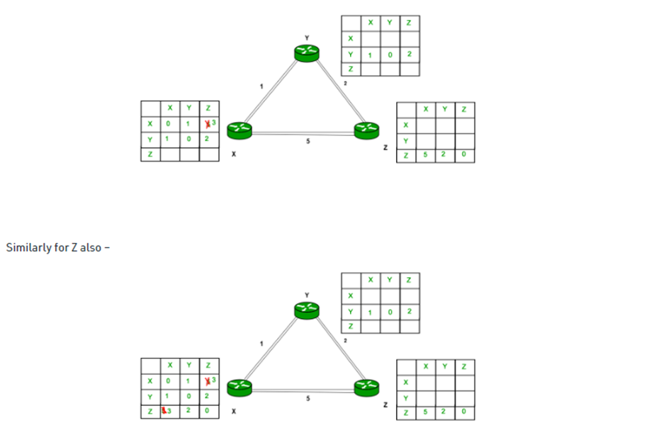
Example – Consider 3-routers X, Y and Z as shown in figure. Each router have their routing table. Every routing table will contain distance to the destination nodes.

Consider router X , X will share it routing table to neighbors and neighbors will share it routing table to it to X and distance from node X to destination will be calculated using bellmen- ford equation.

 Dx(y) = min { C(x,v) + Dv(y)} for each node y ∈ N

As we can see that distance will be less going from X to Z when Y is intermediate node(hop) so it will be update in routing table X.

Advantages of Distance Vector routing –

• It is simpler to configure and maintain than link state routing.

Disadvantages of Distance Vector routing –

• It is slower to converge than link state.
  • It is at risk from the count-to-infinity problem.
  • It creates more traffic than link state since a hop count change must be propagated to all routers and processed on each router. Hop count updates take place on a periodic basis, even if there are no changes in the network topology, so bandwidth-wasting broadcasts still occur.
  • For larger networks, distance vector routing results in larger routing tables than link state since each router must know about all other routers. This can also lead to congestion on WAN links.

Note – Distance Vector routing uses UDP(User datagram protocol) for transportation.

Link State Routing

Link state routing is the second family of routing protocols. While distance-vector routers use a distributed algorithm to compute their routing tables, link-state routing uses link-state routers to exchange messages that allow each router to learn the entire network topology. Based on this learned topology, each router is then able to compute its routing table by using the shortest path computation. 

Features of link state routing protocols – 

• Link state packet – A small packet that contains routing information. 
   
• Link state database – A collection of information gathered from the link-state packet. 
   
• Shortest path first algorithm (Dijkstra algorithm) – A calculation performed on the database results in the shortest path 
   
• Routing table – A list of known paths and interfaces. 

Calculation of shortest path – 
To find the shortest path, each node needs to run the famous Dijkstra algorithm. This famous algorithm uses the following steps: 

• Step-1: The node is taken and chosen as a root node of the tree, this creates the tree with a single node, and now set the total cost of each node to some value based on the information in Link State Database
• Step-2: Now the node selects one node, among all the nodes not in the tree-like structure, which is nearest to the root, and adds this to the tree. The shape of the tree gets changed.
• Step-3: After this node is added to the tree, the cost of all the nodes not in the tree needs to be updated because the paths may have been changed.
• Step-4: The node repeats Step 2. and Step 3. until all the nodes are added to the tree

Link State protocols in comparison to Distance Vector protocols have: 

1. It requires a large amount of memory. 
    
2. Shortest path computations require many CPU circles. 
    
3. If a network uses little bandwidth; it quickly reacts to topology changes 
    
4. All items in the database must be sent to neighbors to form link-state packets. 
    
5. All neighbors must be trusted in the topology. 
    
6. Authentication mechanisms can be used to avoid undesired adjacency and problems. 
    
7. No split horizon techniques are possible in the link-state routing. 
   1. Open Shortest Path First (OSPF) is a unicast routing protocol developed by a working group of the Internet Engineering Task Force (IETF).
   1. It is an intradomain routing protocol.
   1. It is an open-source protocol.
   1. It is similar to Routing Information Protocol (RIP)
   1. OSPF is a classless routing protocol, which means that in its updates, it includes the subnet of each route it knows about, thus, enabling variable-length subnet masks. With variable-length subnet masks, an IP network can be broken into many subnets of various sizes. This provides network administrators with extra network configuration flexibility. These updates are multicasts at specific addresses (224.0.0.5 and 224.0.0.6).
   1. OSPF is implemented as a program in the network layer using the services provided by the Internet Protocol
   1. IP datagram that carries the messages from OSPF sets the value of the protocol field to 89
   1. OSPF is based on the SPF algorithm, which sometimes is referred to as the Dijkstra algorithm
   1. OSPF has two versions – version 1 and version 2. Version 2 is used mostly

OSPF Messages – OSPF is a very complex protocol. It uses five different types of messages. These are as follows:

1. Hello message (Type 1) – It is used by the routers to introduce themselves to the other routers. 
    
2. Database description message (Type 2) – It is normally sent in response to the Hello message. 
    
3. Link-state request message (Type 3) – It is used by the routers that need information about specific Link-State packets. 
    
4. Link-state update message (Type 4) – It is the main OSPF message for building Link-State Database. 
    
5. Link-state acknowledgement message (Type 5) – It is used to create reliability in the OSPF protocol. 

Path Vector Routing

A path-vector routing protocol is a network routing protocol which maintains the path information that gets updated dynamically. Updates that have looped through the network and returned to the same node are easily detected and discarded. This algorithm is sometimes used in Bellman–Ford routing algorithms to avoid “Count to Infinity” problems.

It is different from the distance vector routing and link state routing. Each entry in the routing table contains the destination network, the next router and the path to reach the destination.

Border Gateway Protocol (BGP) is an example of a path vector protocol. In BGP, the autonomous system boundary routers (ASBR) send path-vector messages to advertise the reachability of networks. Each router that receives a path vector message must verify the advertised path according to its policy. If the message complies with its policy, the router modifies its routing table and the message before sending the message to the next neighbor. It modifies the routing table to maintain the autonomous systems that are traversed in order to reach the destination system. It modifies the message to add its AS number and to replace the next router entry with its identification.

Exterior Gateway Protocol (EGP) does not use path vectors.

It has three phases:

1. Initiation
2. Sharing
3. Updating
4. Of note, BGP is commonly referred to as an External Gateway Protocol (EGP) given its role in connecting Autonomous Systems (AS).
5. Communication protocols within AS are therefore referred to as Internal Gateway Protocols (IGP) which contain OSPF and IS-IS among others.
6. This being said, BGP can be used within an AS, which typically occurs within very large organizations such as Facebook or Microsoft.

Hierarchal Routing

In hierarchical routing, the routers are divided into regions. Each router has complete details about how to route packets to destinations within its own region. But it does not have any idea about the internal structure of other regions.

As we know, in both LS and DV algorithms, every router needs to save some information about other routers. When network size is growing, the number of routers in the network will increase. Therefore, the size of routing table increases, then routers cannot handle network traffic as efficiently. To overcome this problem we are using hierarchical routing.

In hierarchical routing, routers are classified in groups called regions. Each router has information about the routers in its own region and it has no information about routers in other regions. So, routers save one record in their table for every other region.

For huge networks, a two-level hierarchy may be insufficient hence, it may be necessary to group the regions into clusters, the clusters into zones, the zones into groups and so on.

Example

Consider an example of two-level hierarchy with five regions as shown in figure −

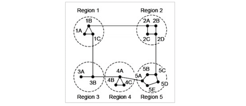
When routing is done hierarchically then there will be only 7 entries as shown below –

Explanation

Step 1 − For example, the best path from 1A to 5C is via region 2, but hierarchical routing of all traffic to region 5 goes via region 3 as it is better for most of the other destinations of region 5.

Step 2 − Consider a subnet of 720 routers. If no hierarchy is used, each router will have 720 entries in its routing table.

Step 3 − Now if the subnet is partitioned into 24 regions of 30 routers each, then each router will require 30 local entries and 23 remote entries for a total of 53 entries.

Example

If the same subnet of 720 routers is partitioned into 8 clusters, each containing 9 regions and each region containing 10 routers. Then what will be the total number of table entries in each router.

Solution

10 local entries + 8 remote regions + 7 clusters = 25 entries

Books on Routing Algorithms